How can a Forecast Time Series be more efficient than Predict Linear Regression?

By, Ahmed Nabil Atwa, Data Scientist | Machine Learning | Deep learning Researcher

Definition of Time Series

Time series is an ordered sequence of values of variables at equally spaced time intervals. 

To understand time series, we shall start with understanding the difference between prediction and forecasting.

• Prediction is a definitive and specific statement that gives you a future perspective depending on a given dataset.
  • For example, the share of this stock will increase in September 2021.
• Forecasting is a probabilistic statement, over a specific time scale.
  • For example, the share of this stock will increase by 30% over the next couple of days.

So, from what we understand, we can see that time series depends on the probability of the observations. Time Series may typically be hourly, daily, weekly, monthly, quarterly and annual.

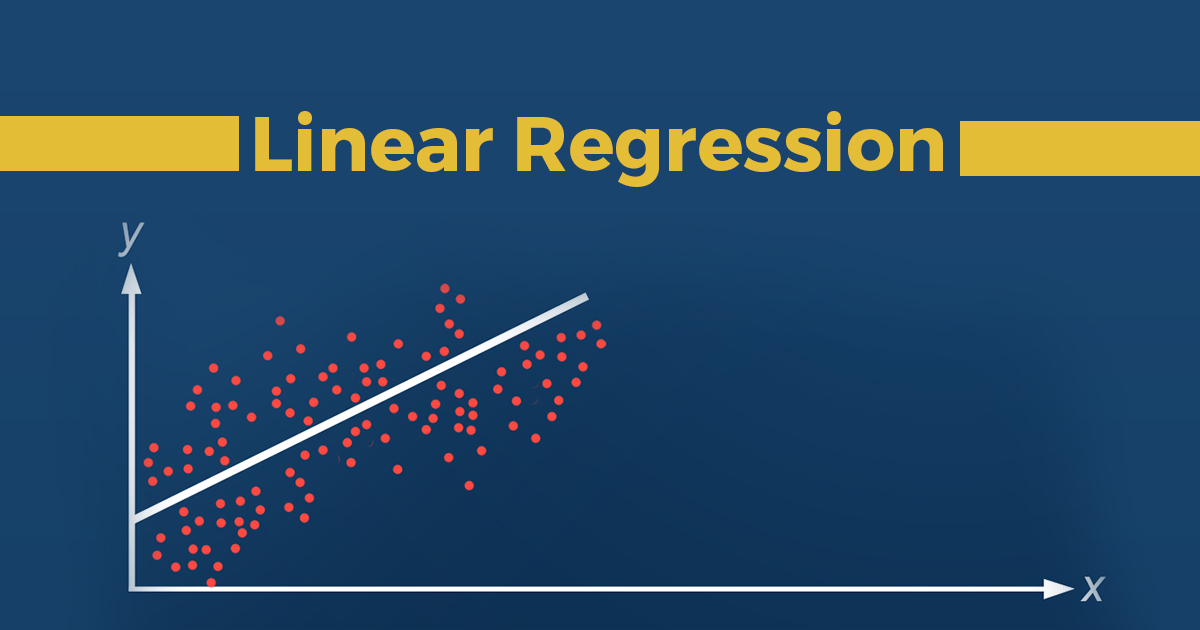
But, linear regression depends on past values to estimate the predicted values, whether it is a future, current or past.

So, How to work on time series forecasting?

There’s a library called sktime.

Anaconda

You can install it using conda:

• conda install -c conda-forge sktime

or with maximum dependencies,

• conda install -c conda-forge sktime-all-extras

or

pip

Using pip, sktime releases are available as source packages and binary wheels. You can see all available wheels here.

• pip install sktime

or, with maximum dependencies,

• pip install sktime[all_extras]

What’s sktime?

• sktime is a unified toolbox for machine learning with time series.
• Time series give rise to multiple learning tasks (e.g. forecasting and time series classification).
• The goal of sktime is to provide all the necessary tools to solve these tasks, including dedicated time series algorithms as well as tools for building, tuning and evaluating composite models.

Many of these tasks are related. An algorithm that can solve one of them can often be re-used to help solve another one, an idea called reduction. sktime’s unified interface allows to easily adapt an algorithm for one task to another.

Forecasting with sktime

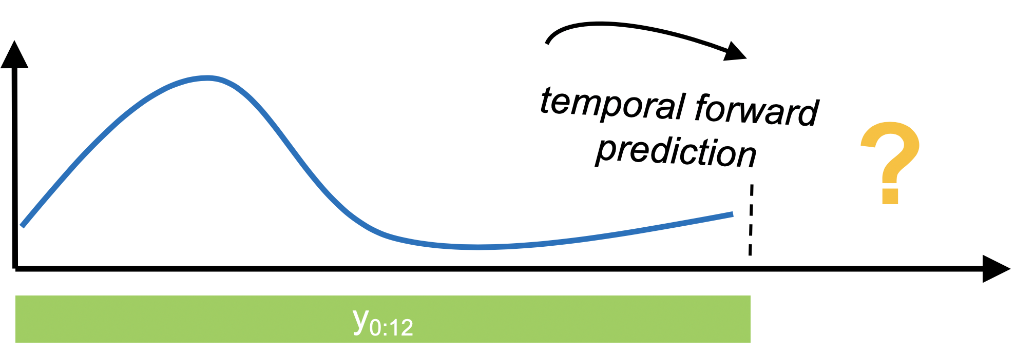
• In forecasting, past data is used to make temporal forward predictions of a time series. This is notably different from tabular prediction tasks supported by scikit-learn and similar libraries.

Time series data and statistical dependence

• An intrinsic characteristic of time series is that observations are statistically dependent on past observations. So, they don’t naturally fit into the standard machine learning setting where we assume to have instances.
• In multivariate data, it is implausible to assume that the different univariate component time series are independent and identically distributed.

sktime uses pandas for representing time series:

• pd.Series for univariate time series and sequences.
• pd.DataFrame for multivariate time series and sequenes.

The Series.index and DataFrame.index are used for representing the time series or sequence index. sktime supports pandas integer, period and timestamp indices.

Structure

For More details, you can check these notebooks and see more about the library and forecasting. In this Article, we will work on using Forecasting.

1. Load dataset.
2. Dat Preprocessing.
   • Data Wrangling.
   • Exploratory Data Analysis.
3. Train Test Split
4. Algorithm Setup.
5. Fit Model.
6. Predict Model.
7. Evaluate Model.

Import Libraries

In [58]:

import pandas as pd
import numpy as np
from sktime.datasets import load_airline
from sktime.utils.plotting import plot_series
import matplotlib.pylab as plt
%matplotlib inline

1. Load dataset

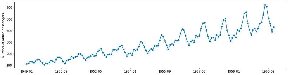
The dataset we have is Box-Jenkins airline dataset, which consists of the number of monthly totals of international airline passengers, from 1949 – 1960. Values are in thousands.In [7]:

series_airline = load_airline()
series_airline

Out[7]:

Period
1949-01    112.0
1949-02    118.0
1949-03    132.0
1949-04    129.0
1949-05    121.0
           ...  
1960-08    606.0
1960-09    508.0
1960-10    461.0
1960-11    390.0
1960-12    432.0
Freq: M, Name: Number of airline passengers, Length: 144, dtype: float64

After loading the data – sktime follows a workflow similar to the sklearn workflow.

The steps in this workflow are as follows:

1. Data Preprocessing.
   • Build specification time points for which forecasts are requested.
   • We can use numpy.array or the ForecastingHorizon object.
2. Split our data into train and test datasets.
3. Building forecasting model and prepare its algorithm.
4. Fitting the forecaster to the data, using the forecaster’s fit method.
5. Making a forecast; using the forecaster’s predict method.
6. Evaluate the forecast model.

2. Data Preprocessing

Display our data to start work on it.In [8]:

# Plotting for visualization
plot_series(series_airline)
plt.show()

In [10]:

# Check the index of the series
series_airline.index

Out[10]:

PeriodIndex(['1949-01', '1949-02', '1949-03', '1949-04', '1949-05', '1949-06',
             '1949-07', '1949-08', '1949-09', '1949-10',
             ...
             '1960-03', '1960-04', '1960-05', '1960-06', '1960-07', '1960-08',
             '1960-09', '1960-10', '1960-11', '1960-12'],
            dtype='period[M]', name='Period', length=144, freq='M')

NOTE:

Generally, users are expected to use the in-built loading functionality of pandas and pandas-compatible packages to load data sets for forecasting, such as read_csv or the Series or DataFrame constructors if data is available in another in-memory format, e.g., numpy.array.

sktime forecasters may accept input in pandas-adjacent formats, but will produce outputs in, and attempt to coerce inputs to, pandas formats.

NOTE: if your favourite format is not properly converted or coerced, kindly consider to contribute that functionality to sktime.

Now, we need to specify the forecasting horizon and pass that to our forecasting algorithm

numpy.arrayIn [12]:

fh = np.arange(1, 37)
fh

Out[12]:

array([ 1,  2,  3,  4,  5,  6,  7,  8,  9, 10, 11, 12, 13, 14, 15, 16, 17,
       18, 19, 20, 21, 22, 23, 24, 25, 26, 27, 28, 29, 30, 31, 32, 33, 34,
       35, 36])

This will ask for monthly predictions for the next three years, since the original series period is 1 month. In another example, to predict only the second and fifth month ahead, one could write:

import numpy as np
fh = np.array([2, 5]) # 2nd and 5th step ahead

ForecastingHorizon

The ForecastingHorizon object takes absolute indices as input, but considers the input absolute or relative depending on the is_relative flag.

ForecastingHorizon will automatically assume a relative horizon if temporal difference types from pandas are passed; if value types from pandas are passed, it will assume an absolute horizon.

To define an absolute ForecastingHorizon in our example:In [13]:

from sktime.forecasting.base import ForecastingHorizon

In [32]:

three_yrs_range = pd.PeriodIndex(pd.date_range('1961-01', periods=36, freq='M'))
fh = ForecastingHorizon(three_yrs_range, is_relative=False)
fh

Out[32]:

ForecastingHorizon(['1961-01', '1961-02', '1961-03', '1961-04', '1961-05', '1961-06',
             '1961-07', '1961-08', '1961-09', '1961-10', '1961-11', '1961-12',
             '1962-01', '1962-02', '1962-03', '1962-04', '1962-05', '1962-06',
             '1962-07', '1962-08', '1962-09', '1962-10', '1962-11', '1962-12',
             '1963-01', '1963-02', '1963-03', '1963-04', '1963-05', '1963-06',
             '1963-07', '1963-08', '1963-09', '1963-10', '1963-11', '1963-12'],
            dtype='period[M]', freq='M', is_relative=False)

ForecastingHorizon-s can be converted from relative to absolute and back via the to_relative and to_absolute methods. Both of these conversions require a compatible cutoff to be passed:In [20]:

cutoff = pd.Period("1960-12", freq='M')
cutoff

Out[20]:

Period('1960-12', 'M')

In [29]:

fh.to_relative(cutoff)

Out[29]:

ForecastingHorizon([ 1,  2,  3,  4,  5,  6,  7,  8,  9, 10, 11, 12, 13, 14, 15, 16, 17,
            18, 19, 20, 21, 22, 23, 24, 25, 26, 27, 28, 29, 30, 31, 32, 33, 34,
            35, 36],
           dtype='int64', is_relative=True)

In [24]:

fh.to_absolute(cutoff)

Out[24]:

ForecastingHorizon(['1961-01-31', '1961-02-28', '1961-03-31', '1961-04-30',
               '1961-05-31', '1961-06-30', '1961-07-31', '1961-08-31',
               '1961-09-30', '1961-10-31', '1961-11-30', '1961-12-31',
               '1962-01-31', '1962-02-28', '1962-03-31', '1962-04-30',
               '1962-05-31', '1962-06-30', '1962-07-31', '1962-08-31',
               '1962-09-30', '1962-10-31', '1962-11-30', '1962-12-31',
               '1963-01-31', '1963-02-28', '1963-03-31', '1963-04-30',
               '1963-05-31', '1963-06-30', '1963-07-31', '1963-08-31',
               '1963-09-30', '1963-10-31', '1963-11-30', '1963-12-31'],
              dtype='datetime64[ns]', freq='M', is_relative=False)

3. Temporal Train and test batch

In [33]:

from sktime.forecasting.model_selection import temporal_train_test_split

In [128]:

y_train, y_test = temporal_train_test_split(series_airline, test_size=36)

We will try to forecast y_test from y_trainIn [38]:

# Plotting for illustration
plot_series(y_train, y_test, labels=['y_train', 'y_test'])
plt.show()
print(f"Y Train Shape: {y_train.shape[0]}\nY Test Shape: {y_test.shape[0]}")

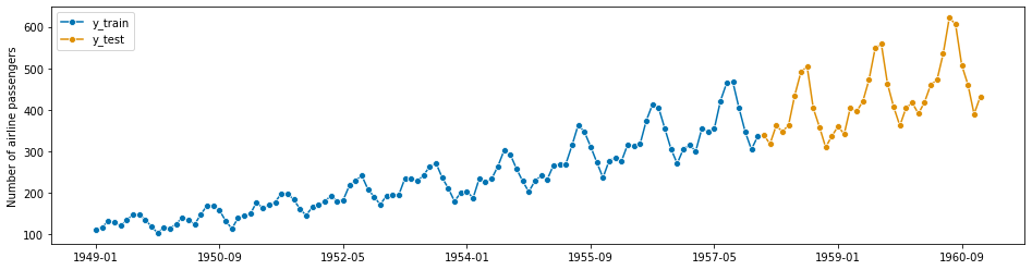
Y Train Shape: 108
Y Test Shape: 36

Why can you use sklearn train_test_split instead of sktime temporal_train_test_split?

In [59]:

from sklearn.model_selection import train_test_split

In [60]:

learn_y_train, learn_y_test = train_test_split(series_airline) 

In [65]:

# Visulaize the data
plot_series(learn_y_train.sort_index(), learn_y_test.sort_index(), labels=['y_train', 'y_test'])
plt.show()

This leads to leakage:

The data you are using to train a machine learning algorithm happens to have the information you’re trying to predict.

But train_test_split(learn_y, shuffle=False) works, Which is what temporal_train_test_split(y) does in sktime.

That’s mean, the data you shuffled has lost the dependencies on its previous variables which connected with.

4. Algorithm setup

In [39]:

from sktime.forecasting.naive import NaiveForecaster

In [41]:

# We can simply take the indices from `y_test` where they already are stored
fh = ForecastingHorizon(y_test.index, is_relative=False)

# apply the algorithm
forecast_model = NaiveForecaster(strategy='last', sp=12)

5. Fitting Model

In [42]:

forecast_model.fit(y_train)

Out[42]:

NaiveForecaster(sp=12)

6. Predict Model

In [129]:

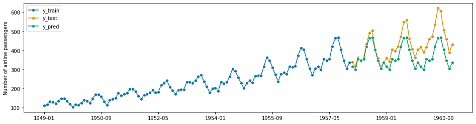
y_pred = forecast_model.predict(fh)

Plotting for illustration

In [45]:

plot_series(y_train, y_test, y_pred, labels=['y_train', 'y_test', 'y_pred'])
plt.show()

7. Evaluate Model

The next step is to specify a forecasting metric. These are functions that return a number when input with prediction and actual series. They are different from sklearn metrics in that they accept series with indices rather than np.arrays. Forecasting metrics can be invoked in two ways:

• using the lean function interface, e.g., mean_absolute_percentage_error which is a python function (y_true : pd.Series, y_pred : pd.Series) -> float
• using the composable class interface, e.g., MeanAbsolutePercentageError, which is a python class, callable with the same signature (*compu

mean_absolute_percentage_error

In [46]:

from sktime.performance_metrics.forecasting import mean_absolute_percentage_error

In [47]:

mean_absolute_percentage_error(y_test, y_pred)

Out[47]:

0.145427686270316

MeanAbsolutePercentageError

In [49]:

from sktime.performance_metrics.forecasting import MeanAbsolutePercentageError

In [50]:

mape = MeanAbsolutePercentageError(symmetric=False)
mape(y_test, y_pred)

Out[50]:

0.13189432350948402

mean_squared_percentage_error

In [66]:

from sktime.performance_metrics.forecasting import mean_squared_percentage_error

In [67]:

mean_squared_percentage_error(y_test, y_pred)

Out[67]:

0.030181651132460994

How ISmile Technologies Help: 

• ISmile Technologies provides advanced machine learning and predictive modeling techniques to analyze and forecast time series data. 
• With its expertise in statistical modeling and time series analysis, ISmile can provide more accurate and reliable forecasts than simple linear regression. 
• ISmile’s forecasting models take into account various factors such as seasonality, trends, and cyclic patterns, which are often overlooked in linear regression. 
• By using machine learning algorithms and advanced statistical models, ISmile can quickly and efficiently process large amounts of data, resulting in more timely and accurate forecasts. 

• In addition to forecasting, ISmile can provide valuable insights and recommendations for businesses to improve their decision-making and optimize their operations. 

ISmile Technologies can help businesses gain a competitive advantage by providing more accurate and efficient time series forecasting than traditional linear regression methods. By leveraging advanced machine learning algorithms and statistical models, ISmile can provide valuable insights and recommendations to optimize business operations and drive growth. 

Summary

• To summarize that, we can say, if your model starts working on observations that depend on time scale – it will be more efficient to use time series forecasting – this will help you to have precise forecasting according to the selected time.
  • For instance, if you’re looking for getting the price of a share over the next day, you will need to use time-series to forecast the share’s price.
• But, If your observations contain only continuous data and you’re looking to predict estimate values, whether it is future, current, or past values.
  • For instance, if you’re looking for getting the prices of the shares in August, you need to give the model the last three months of the observation to analyze it and give the prediction of these shares.

References

• Lecture 13 Time Series Analysis
• Difference between forecast and prediction?
• sktime library examples
• Time Series Analysis in Python
• Introduction to Machine Learning with Time Series || Markus Loning