Dimension Reduction: Methods, components and its projection

Dimension reduction is an unsupervised machine learning technique. So since its an unsupervised, we’re not going to make use of labels. The goal of dimension reduction is to take observations characterized by features and reduce the number of features. The main applications of dimension reduction are to reduce files during the fit method to be easy to transfer or store. Another reason or else the main motivating reason we do it is just for visualization, and the purpose is that it is tough to visualize high dimension datasets.  

These two examples were independent of machine learning; the main reason for dimension reduction regarding machine learning is faster training and predicting times for supervised machine learning models. Reducing the dimensions also helps generate a better, truncated set of new features to represent our data. While lowering the dimension will result in some information loss, the algorithms we will discuss aim to keep this loss minimum.     

Mathematics of Projection 

Dimension reduction techniques work by creating a new set of dimensions and projecting the data to the new space. The process of projecting is matrix multiplication, M’ = MPM′ = MP, wherein M is the matrix of the original data with n observations and p features, M’ is the matrix of the data in new space. P is the matrix that projects the data into a new feature space with p rows and p columns where each column represents a vector in a new dimension. If we only include m columns of matrix P, then the matrix multiplication will project the data onto a lower-dimensional space.  

The matrix with m columns of matrix P is called the truncated form of P, and dimension reduction algorithms work by finding P inscribed within an objective function. Typically constructing the projection matrix P. In such a way, using the truncated form, it can still retain the majority of the information in the data set.   

PCA (Principal Component Analysis) 

PCA is a popular dimension reduction technique in the field of machine learning. It takes a data set characterised by a set of possibly correlated features and generates a new set of uncorrelated features. These new features are going to be based upon the old features so that when we generate these uncorrelated features, then we can only keep a fraction of them (most important ones) that I need to capture a majority of the variation of data set so we can go from let’s say a thousand features to a hundred new features that might capture ninety-ninety five per cent variation of the dataset. So, this is the whole goal of PCA. 

To apply the PCA algorithm, we need to center the dataset (to remove the mean of the dataset) and scaled it to work because PCA does not scale the data automatically. When we use PCA, we will set the number of components so that it gives back a dataset with only that number of components specified earlier when we run it.   

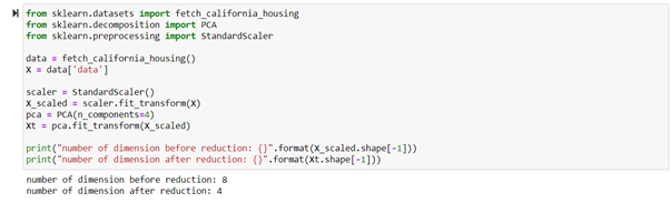
So, when we use the fit method, the transformer learns the matrix P to use for truncating our dataset given the number of components we want to have for our transformed dataset. In the above code, we have gone from 8 to 4 dimensions. So if we’re going to know how much of the original information is retained, we will use explained_variance_ and explained_variance_ratio_. 

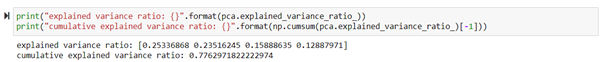
With these four components, we can capture about 77% of the variance of the original full dataset.  

What exactly is happening during the fit method? 

We earlier saw that it’s going to solve for this projection matrix P’ during the fit method, but we haven’t talked about how exactly it is going to solve. Several algorithms solve for the principal components, but a popular one involves applying singular value decomposition (SVD). SVD is an algorithm to decompose a matrix into a product of three matrices. 

 Xc=UΣPTXc=U?PT 

The subscript c is the centred dataset. So by applying SVD on a centred dataset, the matrix P is solved. The matrix Σ is a diagonal matrix; the values along the diagonal will be σi?i, larger the value of σ, the greater the amount of variation exist in that component. Thus, to generate P to truncate the data set, the first m components of P are kept. 

How to choose the number of components? 

The best way to determine a good number of components to use is to construct a plot of the cumulative explained variance versus the number of components. We need to identify when increasing the number of components no longer has an appreciable gain in explained variance, the point of diminishing returns. Identifying this region is accomplished using an “elbow plot”, named because of the resemblance of an arm with a bent elbow. So if we plot the elbow plot for the above example we discussed, it would be something like this, 

From this plot, it appears that we need to use 5 or 6 number of components in order to retain 90% or 95% of the variance respectively. One thing to note is that if we use more features, we are more likely to have a lot of redundant information and correlated features. 

Dimension reduction for visualisation 

One of the primary use of dimension reduction is for the visualisation of high dimension datasets. It is very difficult to visualise more than two or three dimensions. One approach can be to choose two or three variables for plotting, but it will only show the relationship of the data for the selected variables. As we cannot select all the features for visualisation, we can generate two or three new features that capture as much variation as possible.