

Extreme Gradient Boosting (xgboost) is a powerful machine learning algorithm and is one of the popular winning recipes. Over the past few years, predictive modeling has been termed as fast and accurate. Most of the tedious work can be done using this algorithm. Compared to the random forest and neural networks, XGBOOST has better efficiency, accuracy, and feasibility. The latest implementation on xgboost was launched in August 2015. Also, it is 10 times faster than existing gradient boosting implementations.
How to build models using Xgboost on R:
1. Load all the libraries
					library(xgboost)
library(readr)
library(stringr)
library(caret)
library(car)
2. Then load the dataset:
For instance, I have taken bank data to check whether the customer is eligible for a loan or not.
					set.seed(100)
setwd("C:\\Users\\ts93856\\Desktop\\datasource")
# load data
df_train = read_csv("train_users_2.csv")
df_test = read_csv("test_users.csv")

# Loading labels of train data

labels = df_train['labels']
df_train = df_train[-grep('labels', colnames(df_train))]
# combine train and test data
df_all = rbind(df_train,df_test)
3. Cleaning the data & featuring it:
					# clean Variables :  here I clean people with age less than 14 or more than 100
df_all[df_all$age < 14 | df_all$age > 100,'age'] <- -1
df_all$age[df_all$age < 0] <- mean(df_all$age[df_all$age > 0])

# one-hot-encoding categorical features

ohe_feats = c('gender', 'education', 'employer')
dummies <- dummyVars(~ gender +  education + employer, data = df_all)
df_all_ohe <- as.data.frame(predict(dummies, newdata = df_all))
df_all_combined <- cbind(df_all[,-c(which(colnames(df_all) %in% ohe_feats))],df_all_ohe)df_all_combined$agena <- as.fa
4. Now we have to test and run the model:
					xgb <- xgboost(data = data.matrix(X[,-1]),
label = y,
eta = 0.1,
max_depth = 15,
nround=25,
subsample = 0.5,
colsample_bytree = 0.5,
seed = 1,
eval_metric = "merror",
objective = "multi:softprob",
num_class = 12,
nthread = 3
)
5. The last step is to score the test population:
Here you have an object “xgb,” an xgboost model. This is the way to score the test population.
					# predict values in test set
y_pred <- predict(xgb, data.matrix(X_test[,-1]))
Parameters can be used in xgboost:
There are 3 types of parameters:
1. General Parameters – Using to do boosting and the model used are tree or linear model.
2. Booster parameters – Depends on which booster has been chosen.
3. Learning Task parameters – Helps to decide on learning scenarios, like regression tasks.
Advanced functionality of xgboost:
Implementing xgboost is really simple compared to other machine learning techniques. We already have a model, as shown above.
Now let’s find the variable importance in the model and subset our variable list:
					# Lets start with finding what the actual tree looks like
model <- xgb.dump(xgb, with.stats = T)
model[1:10] #This statement prints top 10 nodes of the model

# Get the feature real names
names <- dimnames(data.matrix(X[,-1]))[[2]]

# Compute feature importance matrix
importance_matrix <- xgb.importance(names, model = xgb)

# Nice graph
xgb.plot.importance(importance_matrix[1:10,])

#In case last step does not work for you because of a version issue, you can try following :
barplot(importance_matrix[,1])
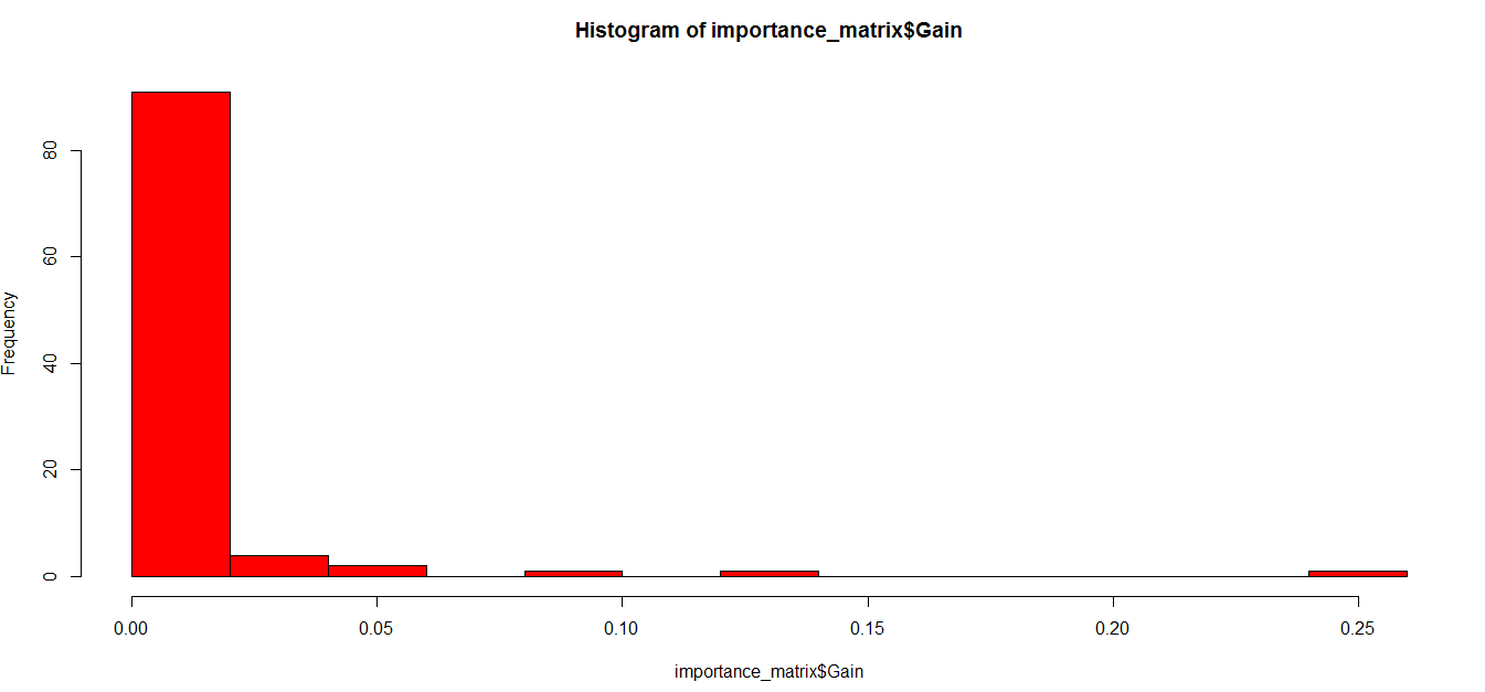
As you can see, there are many variables not worth using in the model, and we are free to remove those variables and run the model again so that we can expect a better accuracy.
Testing whether the result makes sense:
Let’s say age is the variable and the most important one, and there is a simple chi-square test to check whether the variable is important or not.
					test <- chisq.test(train$Age, output_vector)
print(test)
The same process can be done for all the important variables. And we can identify whether the model has identified the important variables or not.