Time Series Analysis

August 31, 2021

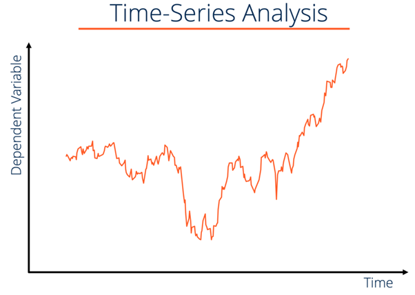
What is Time Series?

A time series is a sequence of measurements of a variable made over time. The typical application of machine learning to a time series is to use past behaviour to make forecasts. Since the time series are usually continuous values, forecasting is a supervised regression problem. Time series differ from the “standard” regression problems because observations are generally not independent and the only piece of data we have is the signal itself. We want to take advantage of the temporal nature of the data without the knowledge of the forces that caused those values.

The general approach when working with a time series is to:

Plot the time series, notice any overall trends and seasonality

Detrend the time series by removing drift and seasonality

Fit a baseline model and calculate the residuals

Analyse the resulting residuals and generate features from the residuals

Train a machine learning model to forecast residuals and add them back to the baseline model.

Components of Time Series

Now you know what is time series is, let’s break down its components. This will be important when we start talking about ARIMA. y(t) =y(t) = drift + seasonal + noise

Drift: An overall trend present in the time series. An example of a drift model is

y(t) = μty(t) = ?t

Seasonality: A periodic behaviour existing in time series. For a given frequency ff, a common model is

y(t) = ∑ (Ansin(2πfnt) + Bncos(2πfnt))y(t) = ∑ (Ansin(2?fnt) + Bncos(2?fnt))

Noise: The part of the time series remaining after removing drift and seasonality. It is residual of a model containing drift and seasonality.

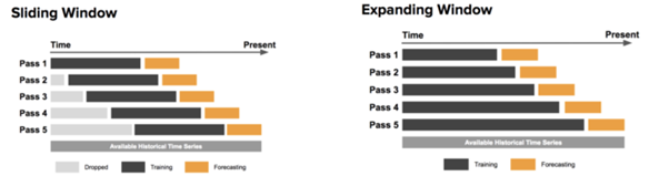
Cross-Validation of Time Series data

Since observations are not independent and we want to use past data to predict future values, we need to apply a slightly different approach when training and testing a machine learning model. Given the temporal nature of the data, we need to preserve order and have the training set occur before the test set. Two standard methods used for cross-validation are:

Sliding Window: The model is trained with data in fixed window size and tested with data in the following window of the same size. Then the window slides where the previous test data becomes the training data and repeated for the number of chosen folds.
Expanding Window: The model is initially trained with windows of the same size as the training window increases in size, containing both the training data and test data.

Stationary Signal

A stationary signal is one in which statistical values such as the mean do not change with time. For our purposes, we are concerned about the special case where the mean, variance, and autocorrelation (explained more later) are not a function of time. This special case is called weakly stationary. Transforming a time series into a stationary process is crucial for time series analysis because a large number of analysis tools assume the process is stationary. It is easy to predict future values if things like the mean and variance stay the same with time.

Let’s take an example of a time series where new values are dependent on the past time series value and a random, uncorrelated noise ?. yt = ⍴yt−1 + ϵt yt = ⍴yt−1 + ?t

The parameter ? scales the contribution of the past value. If ? is uncorrelated and has mean zero, it is referred to as white noise. If the values are sampled from a normal distribution, the white noise is called white Gaussian noise.

Modelling drift, seasonality and noise

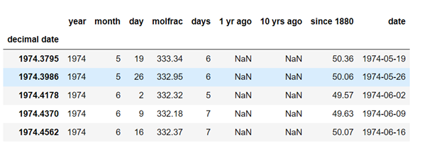
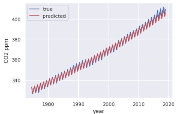
To understand, let’s load a dataset of atmospheric CO2 and plot the time series.

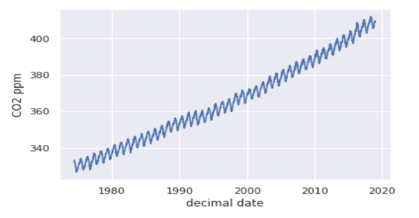
So from the above graph, you can see that atmospheric CO2 levels have been increasing slightly superlinearly. So from this, the choice of drift is quite subjective; that is, we will use a quadratic drift which will be provided from the ‘PolynomialFeatures’ transformer. So the graph you will get is:

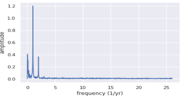
Our next task is to remove the seasonal component of our dataset. Any signal can be represented as a linear superposition of sines and cosines of varying frequencies ff and amplitudes A A and BB, as already mentioned above. So to determine the dominant frequencies that make up a time series, we use Fourier Transform to decompose a signal into a set of frequencies. We are transforming our signal in the time domain into the frequency domain. Here we will use the discrete Fourier Transform as the signal is sampled at discrete points in time. The most common algorithm used to compute the discrete Fourier Transform is the Fast Fourier Transform (FFT) (time complexity = O(nlogn)O(nlogn)). So when you use FFT to determine the contributed frequencies in the given signal, you will get a plot like this:

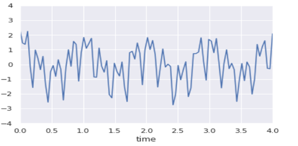
From visual inspection, the signal is derived from y(t) = acos(2πt) + bsin(8πt) + ccos(16πt) + ϵ(t)y(t) = acos(2?t) + bsin(8?t) + ccos(16?t) + ?(t)

So now, let’s formally identify the most dominant frequencies; after inspecting the graph plotted below, you will see two dominant frequencies occurring at once and twice a year. Our updated baseline model will be, y(t) = A +Bt +Ct2+Dsin(2πt) +Ecos(2πt) +Fsin(4πt) +Gcos(4πt)y(t) = A +Bt +Ct2+Dsin(2?t) +Ecos(2?t) +Fsin(4?t) +Gcos(4?t)where t is expressed in units of years.

After incorporating the seasonal components, the graph you will get is

We have a baseline model that works well, but the residuals are not entirely stationary. Our analysis is not done; you can improve the analysis by modelling the noise, the residuals of the baseline model. The autocorrelation (pandas function: autocorrelation_plot) will give you a measure of the persistence of past values; it measures how well correlated a signal is with a lag of copy itself.

Some essential mathematical values that are crucial for understanding the autocorrelation are:

Covariance: A measure of joint variability of two variables.
Variance: A measure of the variability of a variable with itself.
Standard Deviation: The square root of the variance.
Correlation: The normalised covariance ranges from -1 to 1.

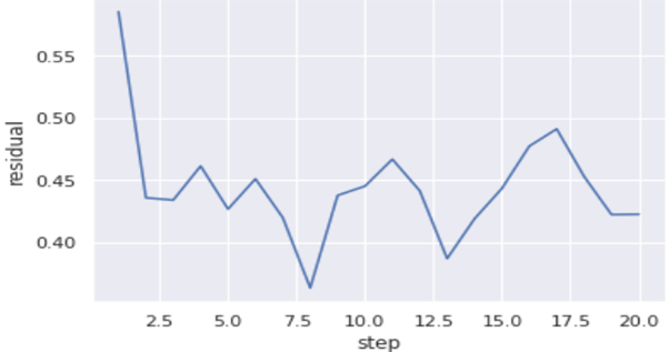
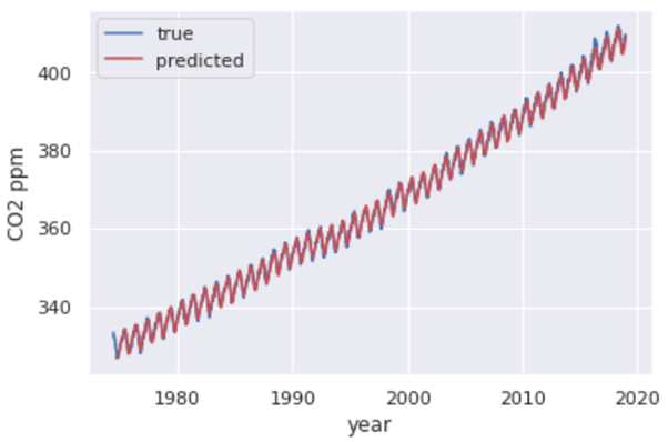
With the baseline model and resulting residuals, you will be able to predict the atmospheric CO2 level 20-30 weeks into the future. So after using the current time step model, the prior residual, the rolling mean of the residual and the rolling mean of the difference of the residual, you will get the graph like this plotted below.

Autoregressive and moving average model

The autoregressive (AR) model of order pp states that the current time series value is linearly dependent on the past ppvalues with some white noise yt =c +α1yt−1+α2yt−2+…αpyt−p+ϵ1=c +Σαpyt−p +ϵtyt =c +?1yt−1+?2yt−2+…?pyt−p+?1=c +??pyt−p +?t,

where αp?pare the model parameters, yt−pyt−pare past time series values, c is a constant, and ϵt?tis white noise. The name autoregressive refers to the model parameters being solved by applying regression with the time series values themselves. Autoregressive models are great at capturing the mean reversion and momentum in the time series since it is based on a window of past values.

Another model is the moving average (MA) model. Despite similar names, the MA model and concept of moving averages are different and should not be confused. The MA model of order ? says that the time series is linearly dependent on current and past shock values or noise, yt =c +β1yt−1+β2yt−2+…βpyt−p+ϵ1=c +Σβpyt−p +ϵtyt =c +?1yt−1+?2yt−2+…?pyt−p+?1=c +??pyt−p +?t,

where βp?p are the model parameter. The MA model captures the persisting effect of shock events on future time series values.

To get the capabilities of both models, AR and MA models are added, forming a more general time series model referred to as the autoregressive and moving average (ARMA) model. The coefficients of the AR models are solved using various methods such as linear least squares regression. MA coefficients are more computationally intensive to solve because shock values are not directly observed, requiring non-linear fitting algorithms. When using ARMA, the order of both AR and MA need to be specified and can be different.

ARIMA

The ARMA model only works for a stationary process. One method to arrive at a stationary process is to apply a difference transformation. In our example of a random walk, the series was not stationary, but the time series of the difference is stationary because it only depends on white Gaussian noise. The autoregressive integrated moving average (ARIMA) model is a general form of ARMA that applies differencing to the time series in the hopes of generating a stationary process.

On using the ARIMA model (using statsmodel package) on the noise/residual of the above data, you will get